Basic Programming#
Introduction#
There are numerous ways to learn the programming language Python. One can find books
Or web-based learning tutorials:
Or via Youtube:
This lecture quickly sketches some key points of the manual, while you should carefully go over Python-Introduction after today’s lecture.
Help System#
The help system for Python is a build-in function named help([object]) with which you can check its usage. Another way to find help is to check each package-documentation you installed.
Vector#
A vector is a collection of elements of the same type, say, integer, logical value, real number, complex number, characters or factor.
Python does not require explicit type declaration. Although, if you want to save a strings, you need " " around your vector
assigns the value on its right-hand side to a self-defined variable name on its left-hand side.
[ ]creates a list of vectorsBinary arithmetic operations
+,-,*and\are performed element by element.Further arithmetic operators: exponends are expressed with
**, and%is the reminder.So are the binary logical operations
&,|,!=,=,<,>,>=,<=.Factor is a categorical number. Character is text.
Example#
Array and Matrix#
To create arrays and matrices, we need to install the package “numpy” as the following:
#Import the NumPy library
import numpy as np
# Import the Pandas library
import pandas as pd
An array is a table of numbers.
A matrix is a 2-dimensional array.
Example#
# Create an array
A = np.array([[1,2,3],[4,5,6]])
A
array([[1, 2, 3],
       [4, 5, 6]])
# Create a matrix
M = np.matrix([[1,2],[3,4]])
M
matrix([[1, 2],
        [3, 4]])
#Shape of matrix
A.shape
(2, 3)
For further readings, please find a list of basic commands in the documentation of NumPy: https://docs.scipy.org/doc/numpy/user/numpy-for-matlab-users.html
OLS-Example#
OLS estimation with one \(x\) regressor and a constant. Graduate textbook expresses the OLS in matrix form \(\hat{\beta} = (X' X)^{-1} X'y.\) To conduct OLS estimation in Python, we literally translate the mathematical expression into code.
Step 1: We need data \(Y\) and \(X\) to run OLS. We simulate an artificial dataset.
# simulate data
import random
np.random.seed(111) # can be removed to allow the result to change
# set the parameters
n = 100
b0 = np.matrix([ [1],[2] ] )
# generate the data
e = np.random.normal(size = (n,1))
X = np.hstack((np.ones((n, 1)), np.random.normal(size = (n, 1))))
y = np.dot(X, b0) + e
Step 2: translate the formula to code
# OLS estimator
bhat = np.dot(np.linalg.inv(np.dot( X.T, X ) ), np.dot( X.T, y ) )
print(bhat)
[[0.99086531]
 [1.92203641]]
Package/Module/Library#
Similar to the packages in R, Python has numerous useful packages/modules/libraries. You have first install the targeted package into the environment (different IDEs have different installing procedures). Then to invoke a module in a certain scripts, use the function import(module_name) as abbr; every time the function of the module is called, use abbr.func_name().
Input and Output#
To read and write csv files in Python, use the pandas library.
Example:#
import pandas as pd
sample_data = pd.read_csv('source.csv')
sample_data = sample_data.dropna()
pd.to_csv(sample_data, file = 'out.csv')
Statistics#
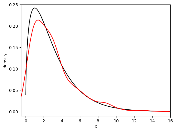
To implement most of the statistical tasks, use the package SciPy. Commonly used probability distributions can be found in the subpackage SciPy.stats. If you hope to draw the kernel density plot for a given set of data, use the seaborn package.
Example:#
# Import Packages
import seaborn as sns
from scipy import stats
import numpy as np
import matplotlib.pyplot as plt


x = np.linspace(0.01, 16, num = 1600)
y = stats.chi2.pdf(x, 3)
z = stats.chi2.rvs(3, size = 1000)

plt.plot(x, y, linestyle = '-', color = 'black')
sns.distplot(z, hist = False, color = 'red')
plt.xlim(-0.5, 16)
plt.ylim(-0.01, 0.25)
plt.xlabel('X')
plt.ylabel('density')
plt.show()
/var/folders/z7/k6ryh25d6jj9s6wh66q1g2hr0000gn/T/ipykernel_54879/3930501868.py:13: UserWarning:

`distplot` is a deprecated function and will be removed in seaborn v0.14.0.

Please adapt your code to use either `displot` (a figure-level function with
similar flexibility) or `kdeplot` (an axes-level function for kernel density plots).

For a guide to updating your code to use the new functions, please see
https://gist.github.com/mwaskom/de44147ed2974457ad6372750bbe5751

  sns.distplot(z, hist = False, color = 'red')

crit = stats.chi2.ppf(q = 0.95, df = 3)
print(len([i for i in z if i > crit]) / len(z))
0.053
User-defined function#
The format of a user-defined function in Python is
def function_name(input): expressions return output
The beginning of the main function is written as follows:
if _name_ == '_main_': expressions function_name
Example:#
If the central limit theorem is applicable, then we can calculate the 95% two-sided asymptotic confidence interval as $\(\left(\hat{\mu} - \frac{1.96}{\sqrt{n}} \hat{\sigma}, \hat{\mu} + \frac{1.96}{\sqrt{n}} \hat{\sigma} \right)\)$ from a given sample. It is an easy job.
#construct confidence interval

def CI(x):
    #x is a vector of random variables
    n = len(x)
    mu = np.mean(x)
    sig = np.std(x)
    upper = mu + 1.96 / np.sqrt(n) * sig
    lower = mu - 1.96 / np.sqrt(n) * sig
    return {'lower': lower, 'upper': upper}
Flow Control#
Flow control is common in all programming languages.
if is used for choice, and for or while is used for loops.
Example#
Calculate the empirical coverage probability of a Poisson distribution of degrees of freedom 2. We conduct this experiment for 1000 times.
import datetime
from scipy import stats

Rep = 1000
sample_size = 100
capture = [0] * Rep


for i in range(Rep):
    mu = 2
    x = stats.poisson.rvs(mu, size = sample_size)
    bounds = CI(x)
    if (bounds['lower'] <= mu and mu <= bounds['upper']):
        capture[i] = 1


print(np.mean(capture))
0.949
Statistical Model#
Statistical models are formulated as y~x, where y on the left-hand side is the dependent variable,
and x on the right-hand side is the explanatory variable.
The OLS function of the package scikit-learn is LinearRegression(). It is called by LinearRegression().
import numpy as np
from scipy import stats
import statsmodels.api as sm

T = 30
p = 2
b0 = np.full([p,1], 1 )

#generate data
x = stats.norm.rvs(size = [T,p])
y = np.dot(x, b0) + stats.norm.rvs(size = [T,1])


#Linear model
model = sm.OLS(y, x)
results = model.fit()
print(results.summary())
                                 OLS Regression Results
=======================================================================================
Dep. Variable:                      y   R-squared (uncentered):                   0.782
Model:                            OLS   Adj. R-squared (uncentered):              0.767
Method:                 Least Squares   F-statistic:                              50.26
Date:                Mon, 22 Jul 2024   Prob (F-statistic):                    5.42e-10
Time:                        14:19:14   Log-Likelihood:                         -38.515
No. Observations:                  30   AIC:                                      81.03
Df Residuals:                      28   BIC:                                      83.83
Df Model:                           2
Covariance Type:            nonrobust
==============================================================================
                 coef    std err          t      P>|t|      [0.025      0.975]
------------------------------------------------------------------------------
x1             0.5901      0.167      3.527      0.001       0.247       0.933
x2             1.2349      0.146      8.439      0.000       0.935       1.535
==============================================================================
Omnibus:                        2.181   Durbin-Watson:                   2.222
Prob(Omnibus):                  0.336   Jarque-Bera (JB):                1.339
Skew:                           0.223   Prob(JB):                        0.512
Kurtosis:                       2.066   Cond. No.                         1.29
==============================================================================

Notes:
[1] R² is computed without centering (uncentered) since the model does not contain a constant.
[2] Standard Errors assume that the covariance matrix of the errors is correctly specified.
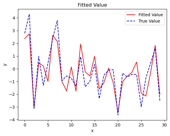
plt.plot(results.fittedvalues, color = 'red', label = 'Fitted Value')
plt.plot(y, color = 'blue', linestyle = 'dashed', label = 'True Value')
plt.title('Fitted Value')
plt.xlabel('x')
plt.ylabel('y')
plt.legend()
plt.show()

The result object is a list containing the regression results. As shown in the results, we can easily read the estimated coefficients, t-test results, F-test results, and the R-sqaure.
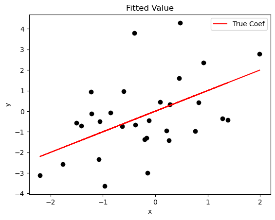
We can plot the true value of \(y\) and fitted value to examine whether the first regressor fits the data.
x0 = x[:,0]
plt.plot(x0, x0*b0.item(0), color = 'red', label = 'True Coef')
plt.scatter(x0, y, color = 'black', marker = 'o')
plt.title('Fitted Value')
plt.xlabel('x')
plt.ylabel('y')
plt.legend()
plt.show()
